UK: IAS 39 Modelling

An example of evaluating the amount of risk and reward transferred and retained in a transfer in accordance with IAS 39 Financial Instruments Recognition and Measurement

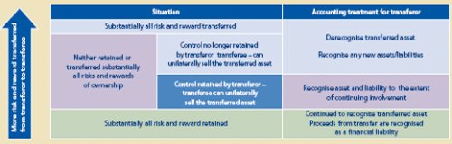
Measuring the relative amount of risk retained by the transferor will be key to determining the accounting treatment for that transfer under IAS 39. The different treatments under IAS 39 are depicted below:

Often it will be obvious whether the transferor has transferred substantially all risks and rewards of ownership or retained substantially all risks and rewards and there will be no need to perform any computations. In other cases, it will be necessary to compute and compare the entity’s exposure to the variability in the present value of the future net cash flows before and after the transfer. The computation and comparison is made using as the discount rate an appropriate current market interest rate. All reasonably possible variability in net cash flows is considered, with greater weight being given to those outcomes that are more likely to occur [IAS 39.22]. This guidance is reminiscent of the principles in FIN 46R, the US consolidation standard applicable to vehicles know as "variable interest entities" found in many securitisation transactions. However, the IASB did not specify what statistic (eg standard deviation, variance, or mean absolute deviation as in FIN 46R) should be used to measure "variability."

The IASB did provide a numerical example to illustrate the application of the continuing involvement approach in IAS 39.AG52. That example assumes, but does not demonstrate, the conclusion that the transferor has passed some significant risk and rewards of ownership of the transferred assets (eg prepayment risk) while continuing to retain some significant risks and rewards (eg credit risk). The worksheet below shows one method, based on the standard deviation statistic¹, which might be used when calculations are required. The calculations require information about various possible future scenarios that are not included in the IAS 39 example. So we needed to imagine the necessary data, while trying to keep it as consistent as possible to what information was given in IAS 39.AG52. In real life, one would probably need more than four scenarios and they should be based on real, supportable expectations and experience. With that said, the assumed scenarios are as follows:

Scenario 1: Prepay immediately – All loans prepay all outstanding principal of £10,000 immediately after the closing of the securitisation. There are no defaults and no interest has accrued since the closing date. The senior investors are entitled to 90% of the principal proceeds, or £9,000 and the transferor is entitled to the remaining £1,000. Probability = 20%

Scenario 2: Prepay in one year – All loans prepay all outstanding principal and accrued interest of £1,000 on the coupon payment date, which is the first anniversary of the securitisation closing. There are no defaults. The senior investors are entitled to 90% of the principal proceeds plus interest at the rate of 9.5% thereon for a total of £9,855 and the transferor is entitled to the remaining £1,145. Probability = 30%

Scenario 3: Mature in two years – All loans run to their contractual maturity at the end of two years. They pay timely the £1,000 coupon interest payment due on the first anniversary of the securitisation closing and all outstanding principal and accrued interest of £1,000 on the maturity date, which is the second anniversary of the securitisation closing. There are no defaults. The senior investors are entitled to one coupon payment of £855 and a final payment of £9,855 and the transferor is entitled to the remaining coupon payment of £145 and final payment of £1,145. Probability = 30%

Scenario 4: Default in one year – All loans default on all outstanding principal and accrued interest on the coupon payment date, which is the first anniversary of the securitisation closing. Through immediate foreclosure and sale of the collateral properties, a total of £10,741 is recovered and applied to repay principal and accrued interest, first to the senior bond, then the subordinated bond. No recovery proceeds are available to the IO strip. The senior investors are entitled to the same £9,855 as in Scenario 2, while the transferor is receives the remaining £886. Probability = 20%

IAS 39 does not differentiate based on how the risk is allocated among the transferees. Similarly, IAS 39 does not care how or in how many tranches the transferor’s risk is retained. Therefore, the analysis can be simplified by dividing the asset cash flows for each scenario into two buckets – the total amount attributable to the transferor and everything else, which represents the net amount attributable to all the transferees taken as a group.

That method is illustrated in the tables below. Obviously we had to reverse engineer the assumptions in order to make this example that tie to the IAS 39 example. Please forgive the occasional liberty we took in rounding trying to keep the numbers as simple as possible.

Notice that the sum of the standard deviations of the Transferred Senior portion and the Retained Subordinated and IO portions add up to more than the standard deviation of the loans as a single portfolio. Try to visualize this effect with the following picture of a triangle. We us arrows for the sides of the triangle, because risk has a direction associated with it (eg a long or short position). The diagram shows that in total, we start at the same beginning spot and arrive at the same end point before and after the transaction. The paths are simply different.

One way to evaluate the amount of risk transferred would be to sum up the total risk exposure of the transferor after the transaction and the net risk exposure of the transferees as a group to create a new, larger denominator. Then you could divide the transferor’s total risk after the transaction by that sum. This is a simplified method, and it could be argued is an acceptable approach. However, you could argue that because IAS 39 focuses on the proportion of the risk of ownership of the assets that has been transferred or retained, not the absolute amount of risk exposure of the transferor or transferee, an alternative approach that is described below can be applied.

This distinction is important, because risk does not add or subtract in simple, arithmetic ways. The portfolio diversification effect of the loans as a group reduced the total risk of the portfolio to something less than the arithmetic sum of the risks of each loan. The subordination structure of the transaction acts in a similar fashion, but in the opposite direction. Rather than reducing risk through diversification, it increases risk by introducing to both the transferor and transferees as a group an equal and offsetting new risk that is completely uncorrelated with the aggregate asset portfolio risk. In essence, the transferor and transferee have made a small "side bet" using a portion of the asset portfolio as the amount of the wager. Visualize this by breaking the previous diagram into two parts.

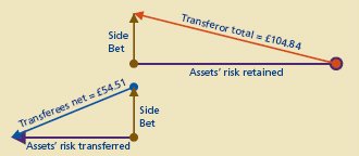
Again, each diagram shows the same beginning and end to represent the total risk to the transferor and the net risk to the transferees as a group. It also reveals the portion of the risk of the assets retained and transferred. If we knew how the asset portfolio risk correlated with the total risk to the transferor or the net risk to the transferees as a group, it would be a simple matter to measure the numerical amount of the asset risk retained and transferred. A simple multiplication of the transferor’s total risk or the transferees’ net risk amounts by their individual correlation coefficients (their respective r statistics) will yield the answer.

However, calculating those correlation coefficients is a tedious and cumbersome numerical exercise. Readers that remember their trigonometry lessons from school will recognise the multiplication step described above using the correlation coefficient as the same multiplication that could be done using the cosine of the angle between a leg and hypotenuse of a right triangle. In this case, the cosine of the angle between the two arrows with the same starting spots in the transferor diagram would represent the transferor’s correlation coefficient. Similarly, the cosine of the angle between the two arrows with the same ending points in the transferee diagram would represent the correlation coefficient of the transferees as a group. Using that idea and some more trigonometry, you can prove a pair of easier formulas to calculate the percentage of asset risk retained and transferred that use only the risk amounts we have already calculated. The formulas use the length of each line squared. Fortunately, if our arrows represent standard deviation statistics, the squared amounts are the previously calculated variance statistics (abbreviated as Var below). The formulas work out to:

IAS 39 does not did establish any bright-line guidance on the cutoff levels for what represents "substantially all". If the transferor believes that something in the region of 80% to 90% it equivalent to "substantially all", then in this hypothetical case the entity would conclude that the transferor had neither transferred nor retained substantially all of the risk and reward of the portfolio following transfer.

Footnotes

The content of this article is intended to provide a general guide to the subject matter. Specialist advice should be sought about your specific circumstances.